Wave Propagation On a Transmission Line
If an electrical line is long enough (\(\frac{l}{\lambda}\gtrapprox{}0.01\)), the effects of the length must be taken into account. We call such lines TEM transmission lines, and they consist of two conductors separated by a dielectric material (for example, a coaxial cable).
The Telegrapher’s Equations
To try and understand the behavior of voltage and current along transmission lines, we divide one into \(n\) two port networks of length \(\Delta{}z\), one of which is shown below.
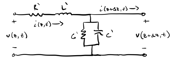
The circuit parameters shown depend on the geometry of the transmission line and are defined as:
- \(R'\) – the distributed resistance of the line in Ohms per meter.
- \(L'\) – the distributed inductance of the line in Henries per meter.
- \(C'\) – the capacitance between the two conductors of the line in Farads per meter.
- \(G'\) – the conductance of the dielectric between the conductors in Siemens per meter.
These parameters depend on the geometry and the materials of the line itself. KVL around the outer loop obtains
\[\begin{align*} v(z,t)-v(z+\Delta{}z,t)=R'\Delta{}zi(z,t)+L'\Delta{}z\pderiv{i(z,t)}{t}\\ -\frac{v(z+\Delta{}z,t)-v(z,t)}{\Delta{}z}=R'i(z,t)+L'\pderiv{i(z,t)}{t} \end{align*}\]Letting \(n\) grow to infinity, the equation becomes the first of the Telegrapher’s Equations, describing voltage.
\[\begin{equation} -\pderiv{v(z,t)}{z}=R'i(z,t)+L'\pderiv{i(z,t)}{t} \label{eq:telegraphers_voltage} \end{equation}\]A similar process with KCL down the shunt gives
\[\begin{align*} i(z,t)-i(z+\Delta{}z,t)&=G'\Delta{}zv(z,t)+C'\pderiv{v(z,t)}{t}\\ -\frac{[i(z+\Delta{}z,t)-i(z,t)]}{\Delta{}z}&=G'v(z,t)+C'\pderiv{v(z,t)}{t}\\ \end{align*}\]Again letting \(n\) grow infinitely large yields the second Telegrapher’s Equation, describing current.
\[\begin{equation} -\pderiv{i(z,t)}{z}=G'v(z,t)+C'\pderiv{v(z,t)}{t} \label{eq:telegraphers_current} \end{equation}\]Wave Propagation
One fruitful avenue of analysis is the behavior of sinusoidal steady-state voltages and currents along transmission lines. To that end, we use the phasor form of the Telegrapher’s Equations.
\[\begin{equation} -\deriv{\tilde{V}(z)}{z}=\tilde{I}(z)(R'+j\omega{}L') \label{eq:telegraphers_voltage_phasor} \end{equation}\] \[\begin{equation} -\deriv{\tilde{I}(z)}{z}=\tilde{V}(z)(G'+j\omega{}C') \label{eq:telegraphers_current_phasor} \end{equation}\]Taking the derivative with respect to \(z\) of both sides of Eq. (\ref{eq:telegraphers_voltage_phasor}) and substituting in Eq. (\ref{eq:telegraphers_current_phasor}) for current, we get
\[-\frac{\partial{}^2\tilde{V}(z)}{\partial{}z^2}=-\tilde{V}(z)(G'+j\omega{}C')(R'+j\omega{}L')\]A little bit of rearrangement yields a wave equation
\[\begin{equation} \frac{\partial{}^2\tilde{V}(z)}{\partial{}z^2}-\gamma^2\tilde{V}(z)=0 \label{eq:voltage_wave} \end{equation}\]where \(\gamma=\sqrt{(R'+j\omega{}L')(G'+j\omega{}C')}=\alpha+j\beta\) is defined as the propagation constant of the transmission line. It consists of a real part, an attenuation constant \(\alpha\), and a phase constant \(\beta\). A similar procedure obtains the corresponding current wave equation.
\[\begin{equation} \frac{\partial{}^2\tilde{I}(z)}{\partial{}z^2}-\gamma^2\tilde{I}(z)=0 \label{eq:current_wave} \end{equation}\]The general solution of these equations is well known, and takes the form
\[\begin{equation} \color{blue}{\tilde{V}(z)=V_0^+e^{-\gamma{}z}+V_0^-e^{\gamma{}z}} \label{eq:voltage_general_solution} \end{equation}\] \[\begin{equation} \label{eq:current_general_solution} \color{blue}{\tilde{I}(z)=I_0^+e^{-\gamma{}z}+I_0^-e^{\gamma{}z}} \end{equation}\]If we return to the time domain, it is clear these solutions describe the sum of waves traveling in opposing directions, a phenomena known as a standing wave, whose forward propagating waves have amplitudes \(V_0^+\) and \(I_0^+\) and whose backward propagating waves have amplitudes \(V_0^-\) and \(I_0^-\).
Characteristic Impedance
We now have equations that describe the behavior of voltage and current waves on a transmission line. But we still have four unknown amplitudes.
We can reduce the number of unknowns to two by relating the voltage and current amplitudes. To do this, we substitute Eq. (\ref{eq:voltage_general_solution}) into Eq. (\ref{eq:telegraphers_voltage_phasor}) and solve for \(\tilde{I}(z)\).
\[\begin{align*} \tilde{I}(z)&=I_0^+e^{-j\gamma}+I_0^-e^{j\gamma}\\ &=\frac{\gamma}{R'+j\omega{}L'}(V_0^+e^{-\gamma{}z}-V_0^-e^{\gamma{}z})\\ \end{align*}\]Comparing the amplitudes of voltage and current, it is clear that
\[\begin{equation} V_0^+=\frac{I_0^+}{Z_0}\qquad{}V_0^-=-\frac{I_0^-}{Z_0} \end{equation}\]where \(Z_0\) is defined as the characteristic impedance and given by
\[\begin{equation} Z_0=\frac{R'+j\omega{}L'}{\gamma}=\sqrt{\frac{R'+j\omega{}L'}{G'+j\omega{}C'}} \label{eq:characteristic_impedance_general} \end{equation}\]We can now define Eq. (\ref{eq:current_general_solution}) in terms of the characteristic impedance.
\[\begin{equation} \color{blue}{\tilde{I}(z)=\frac{V_0^+}{Z_0}e^{-\gamma{}z}-\frac{V_0^-}{Z_0}e^{\gamma{}z}} \label{eq:current_solution_characteristic_impedance} \end{equation}\]The Lossless Case
A well designed transmission line uses conductors with high conductivity and dielectrics with high resistivity, making \(R'\) and \(G'\) very small. In the ideal case, \(R'=G'=0\) and the line is considered “lossless”. The propagation constant of such a line reduces to
\[\begin{equation} \gamma=\alpha+j\beta=j\omega{}\sqrt{L'C'} \end{equation}\]which implies that \(\alpha=0\) and \(\beta=\omega{}\sqrt{L'C'}\), or \(\gamma=j\beta\). Thus Eqs. (\ref{eq:voltage_general_solution}) and (\ref{eq:current_solution_characteristic_impedance}) reduce to
\[\begin{equation} \color{blue}{\tilde{V}(z)=V_0^+e^{-j\beta{}z}+V_0^-e^{j\beta{}z}} \label{eq:voltage_wave_lossless} \end{equation}\] \[\begin{equation} \color{blue}{\tilde{I}(z)=\frac{V_0^+}{Z_0}e^{-j\beta{}z}-\frac{V_0^-}{Z_0}e^{j\beta{}z}} \label{eq:current_wave_lossless} \end{equation}\]Similarly, the characteristic impedance of a lossless line is given by
\[\begin{equation} Z_0=\sqrt{\frac{L'}{C'}} \label{eq:characteristic_impedance_lossless} \end{equation}\]The fact that a wave’s velocity is given by \(u_p=\frac{\omega}{\beta}\) implies that, in the case of a lossless line, the phase velocity is given by
\[u_p=\frac{\omega}{\beta}=\frac{\omega}{\omega{}\sqrt{L'C'}}=\frac{1}{\sqrt{L'C'}}\]Thus, the velocity of the wave is independent of its frequency. In this way, dispersion (where different frequencies that make up a signal travel at different speeds and therefore arrive at different times, causing distortion) is avoided.
Interestingly, the condition known as the Heaviside Condition, satisfied if \(\frac{G'}{C'}=\frac{R'}{L'}\), also eliminates dispersion. Given the Heaviside Condtion,
\[\begin{align*} \gamma&=\sqrt{(R'+j\omega{}L')(G'+j\omega{}C')}\\ &=\sqrt{L'C'(\frac{R'}{L'}+j\omega{})(\frac{G'}{C'}+j\omega{})}\\ &=\sqrt{R'G'}+j\omega{}\sqrt{L'C'}\\ &=\alpha+j\beta\\ \end{align*}\]Again, the velocity \(u_p=\frac{\omega}{\beta}\) does not depend on frequency, and the the line is known as “distortionless”.
Reflection Coefficient
Limiting ourselves to the lossless case, we apply a boundary condition at the load in order to relate the amplitudes of the forward and backward propagating waves, also known as the incident wave and reflected wave. For convenience, we define the load to be at \(z=0\).
With this in mind, the impedance at the load is
\[Z_L=\frac{\tilde{V}(0)}{\tilde{I}(0)}=Z_0\frac{V_0^++V_0^-}{V_0^+-V_0^-}\]Solving for the ratio of the amplitudes of the incident and reflected waves yields the the voltage reflection coefficient at the load, defined as
\[\begin{equation} \Gamma_L=\frac{V_0^-}{V_0^+}=\frac{Z_L-Z_0}{Z_L+Z_0} \label{eq:reflection_coefficient_load} \end{equation}\]Since \(Z_L\) is in general a complex number, \(\Gamma_L=\vert{}\Gamma_L\vert{}e^{j\theta_{\Gamma}}\). If a load is matched, \(Z_L=Z_0\) and \(\Gamma_L=0\); there is no reflection on the line. If \(Z_L=0\) (a short circuit), \(\Gamma=-1\). If \(Z_L=\infty\) (an open circuit), then \(\Gamma=1\).
Using Eqs. (\ref{eq:voltage_wave_lossless}) and (\ref{eq:reflection_coefficient_load}), we can now define our wave equations with just one unknown, namely \(V_0^+\).
\[\begin{equation} \color{blue}{\tilde{V}(z)=V_0^+(e^{-j\beta{}z}+\Gamma_L{}e^{j\beta{}z})} \label{eq:voltage_wave_gamma} \end{equation}\] \[\begin{equation} \color{blue}{\tilde{I}(z)=\frac{V_0^+}{Z_0}(e^{-j\beta{}z}-\Gamma_L{}e^{j\beta{}z})} \label{eq:current_wave_gamma} \end{equation}\]The Last Unknown
In order to solve for \(V_0^+\), we need to apply another boundary condition, this time at the source. Taking the wave impedance, or the impedance at a point \(z\) on the line, as the ratio of Eqs. (\ref{eq:voltage_wave_gamma}) and (\ref{eq:current_wave_gamma}), we have
\[\begin{align*} Z(z)&=\frac{\tilde{V}(z)}{\tilde{I}(z)}\\ &=Z_0\frac{e^{-j\beta{}z}(1+\Gamma_L{}e^{j2\beta{}z})}{e^{-j\beta{}z}(1-\Gamma_L{}e^{j2\beta{}z})}\\ &=Z_0\frac{1+\Gamma_z}{1-\Gamma_z}\\ \end{align*}\]where \(\Gamma_z=\Gamma_Le^{j2\beta{}z}\), which is \(\Gamma_L\) phase shifted by \(2\beta{}z\) toward the source. The input impedance, or the impedance of a line of length \(l\) at \(z=-l\), is therefore
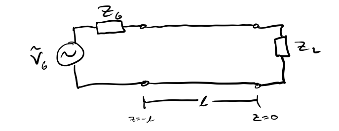
\[Z_{in}=Z(-l)=Z_0\frac{1+\Gamma_L{}e^{-j2\beta{}l}}{1-\Gamma_L{}e^{-j2\beta{}l}}\]The input impedance and the source impedance (as shown in Figure 2) therefore form a voltage divider, expressed by
\[\begin{equation} \tilde{V}(l)=\frac{\tilde{V}_GZ_{in}}{Z_G+Z_{in}} \label{eq:input_voltage} \end{equation}\]The voltage at \(z=-l\) can also be expressed through Eq. (\ref{eq:voltage_wave_gamma}), and when combined with Eq. (\ref{eq:input_voltage}), give us an expression for \(V_0^+\).
\[\begin{equation} V_0^+=(\frac{\tilde{V}_GZ_{in}}{Z_G+Z_{in}})(\frac{1}{e^{j\beta{}l}+\Gamma_Le^{-j\beta{}l}}) \label{eq:incident_wave_amplitude} \end{equation}\]Substituting this equation into Eq. (\ref{eq:voltage_wave_gamma}) yields the final solution to the voltage and current waves along a transmission line of length \(l\), depending only on \(l\) and the parameters of the line \(R'\), \(G'\), \(L'\), and \(C'\).
\[\begin{equation} \color{blue}{\tilde{V}(z)=(\frac{\tilde{V}_GZ_{in}}{Z_G+Z_{in}})(\frac{1}{e^{j\beta{}l}+\Gamma_Le^{-j\beta{}l}})(e^{-j\beta{}z}+\Gamma_L{}e^{j\beta{}z})} \label{eq:voltage_final_solution} \end{equation}\] \[\begin{equation} \color{blue}{\tilde{I}(z)=\frac{1}{Z_0}(\frac{\tilde{V}_GZ_{in}}{Z_G+Z_{in}})(\frac{1}{e^{j\beta{}l}+\Gamma_Le^{-j\beta{}l}})(e^{-j\beta{}z}+\Gamma_L{}e^{j\beta{}z})} \label{eq:current_final_solution} \end{equation}\]